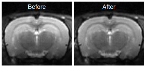
The Filtering tool offers a variety of smoothing filters with configurable input parameters and can be applied to any of the loaded images.
Getting There
The Filtering tool can be accessed via the tool pull-down menu on VivoQuant’s front panel.

Using the Tool
Upon selecting the tool, the Filtering operator window is displayed.
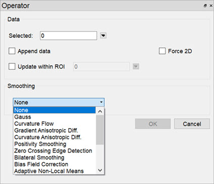
Using this tool, any loaded data can be selected for smoothing via the Data Selector Widget.
Select the desired smoothing algorithm from the available options in the Smoothing drop-down menu. Use the parameter fields to set appropriate values. The effect of the chosen smoothing filter will be previewed in 2D in the slice views. To remove the 2D preview, go back to None in the drop-down menu of smoothing filters.
Currently available filters include:
- Gaussian Smoothing
- Curvature Flow
- Gradient Anisotropic Diffusion
- Curvature Anisotropic Diffusion
- Positivity Smoothing (to remove negativity from FBP reconstructions)
- Zero Crossing Edge Detection
- Bilateral Smoothing
- Bias Field Correction
Each filter uses a different subset of the configurable parameters. See the table below if parameters other than the default settings are desired.
| Parameter | Description | Used by | Default Value |
|---|---|---|---|
| FWHM | Full-width half-maximum kernel size | Gauss, Zero Crossing Edge Detection | 1.00mm |
| Conductance | Parameter governing sensitivity to edge contrast | Gradient Anisotropic Diffusion, Curvature Anisotropic Diffusion | 1 |
| Iter | Number of iterations | Curvature Flow, Gradient Anisotropic Diffusion, Curvature Anisotropic Diffusion, Positivity Smoothing | 5 |
| CutOffFrac | If the fraction of voxels that are negative falls below this value, further iterations of the filter will not be performed. | Positivity Smoothing | 0.005 |
| Time Step | Stepsize, effectively analogous to kernel width | Curvature Flow, Gradient Anisotropic Diffusion, Curvature Anisotropic Diffusion | 0.125 |
| Max Error | Difference between the area under the discrete Gaussian curve and the area under the continuous Gaussian | Zero Crossing Edge Detection | 0.5 |
| Range Sigma | The standard deviation of the gaussian blurring kernel in the image range. Units are intensity. | Bilateral Smoothing | 50 |
| Domain Sigma | The standard deviation of the gaussian blurring kernel in each dimensional direction. Units match image spacing units. | Bilateral Smoothing | 4 |
The smoothing function is executed by left-clicking on OK. Depending on the image size and filter selected, this may take several seconds. Once the smoothing function is applied, any subsequent operations will be based on the smoothed images.
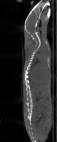
Each filter will have different edge-preserving and noise-reduction properties. Choose the one that best suits your application.
| No Smoothing | Gauss | Curvature Flow | Gradient Anisotropic Diffusion | Curvature Anisotropic Diffusion |
|---|---|---|---|---|
 |
 |
 |
 |
 |
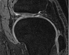
The bilateral smoothing filter could take several minutes for large images in 3D, especially for greater values of domain sigma. Check the Force 2D option to speed up this filter.
| No Filtering Applied | Various Bilateral Smoothing Parameters |
|---|---|
 |
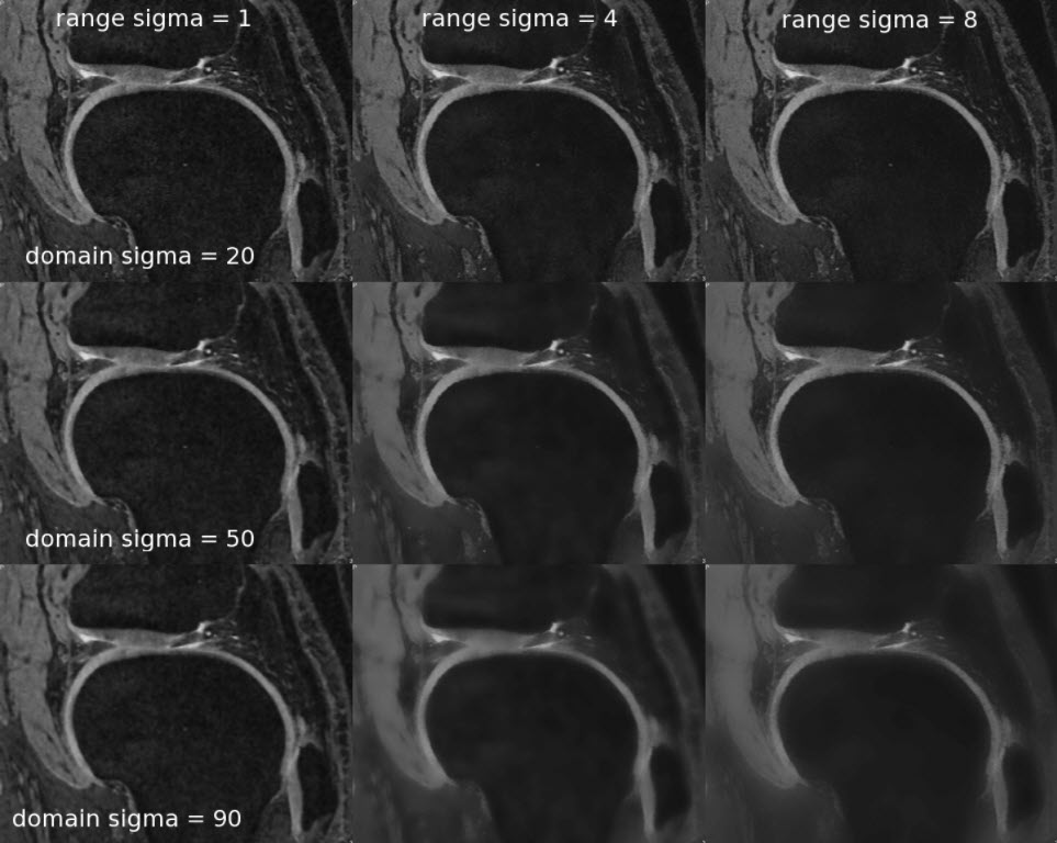 |
The positivity smoothing filter will also typically take longer to run than the other smoothing filters, up to several minutes for larger images. This filter was specially designed to redistribute the activity across neighboring voxels such that the total sum of the image is preserved but the number of voxels with negative values is reduced. It is intended to be used to correct images reconstructed with FBP.
Bias Field Correction
Intensity gradient artifacts in magnetic resonance imaging can often cause difficulties with automated segmentation and analysis tools that rely on intensity contrasts, not to mention the detriment to qualitative appearance. The Bias Field Correction filter implements the N3 bias correction algorithm (Tustison 2010) to estimate the gradient field present in the image and uses this filter to normalize each voxel of the image. Due to the higher performance cost, a preview of its filtering is not available but the filtering can be applied via the filtering operator. The user may optionally adjust the field smoothness to avoid or allow high spatial frequency corrections and also append the estimated bias field as an image to the data manager.
